I made this page for the SPR course in the Summer term 2015. I am not responsible for the course in 2016 or later, and cannot give guarantees with respect to correctness or relevance of this page's contents for the current lecture period.
--Nikolaus MayerPart (b)
If you want to do this exercise in Matlab, reuse your image reading code from exercise 10. For C++, there are many frameworks for working with images, e.g. OpenCV, CImg (which is only a single header file and does not have to be installed!) or the CTensor class that we provide with the exercise material (it offers limited functionality but has everything we need here). Reading the images in pure C++ quickly gets ugly: The Tsukuba images have a binary data blob (magic number P6, see http://paulbourke.net/dataformats/ppm/), and additionally the image header may contain comments. If you want to use Python, there's PIL (available via the packages python-pil resp. python3-pil).
The quality of your results will very much depend on your parameters. Experiment!
This exercise has immense potential for code optimization. Depending on your language of choice, your programming proficiency and the depth of your understanding of this algorithm, your runtime may be as long as ten minutes... or as short as ten milliseconds. How fast are you?
The "Tsukuba" stereo pair is arguably one of the most well-known datasets in this field. Another set is "Venus" (left image, right image) which has the same disparity range but is much more challenging to the human eye (the Tsukuba scene is very natural). A very recent dataset is "Couch" (left image, right image). It is available in multimegapixel resolution, but our scanline method really begins to show its limitations there.
Part (a):
To "visualize the linear subspace", note that the first principal component is the direction vector of this sought subspace. Adding this vector to the mean of the data points gives you points on the subspace which you can use with the plot(..) command.
Part (b):
Use only the images 1 to 36 (or 2 to 37, alternatively): dino1.jpg and dino37.jpg are exactly the same file. Exact duplicates in data are the source of all sorts of mayhem, so let's not ask for trouble with zero-distances and all that.
Does it matter how you transform the images into vectors? I.e., does the ordering of the elements have any effect at all? If not, why? If yes, is it important? What about the color ordering within each RGB pixel?
What is the dimensionality of the dino data? And... what is its intrinsic dimensionality?
Hint: You have to look at and think about the images for the second answer, but not for the first one.
Here's a code snippet to read the dino images and make a matrix image_vectors of column vectors:
%%
%% Load images
%%
image_vectors = [];
N = 36;
for i = 1:N,
    %% Format image file name
    image_filename = sprintf('dino%d.jpg', i);
    fprintf('Reading %s (%d/%d)\n',image_filename,i,N);
    %% Read image as 3d matrix (y*x*rgb)
    dino_image = im2single(imread(image_filename));
    %% Reshape image into vector
    number_of_elements = prod(size(dino_image));
    dino_image_as_vector = reshape(dino_image, number_of_elements, 1);
    %% Add new image vector to collection
    image_vectors = [image_vectors dino_image_as_vector];
end;
The im2single function converts the image data from its default uint8 data type to float numbers (the vector length norm does not work on integers). It also normalizes the numeric range from [0, 255] to [0.0, 1.0], but that's not important here.
The dijkstra(..) function in the linked file takes three parameters (contrary to its description!):
matriz_costo is our euclidean distances matrix
s is the index of the source point
d is the index of the target point
The function returns two elements:
sp is the shortest path across the node graph (we don't need this)
spcost is the cost of the shortest path
Remember to correctly initialize the distances matrix for this algorithm!
To cut the runtime of your algorithm (almost) in half, remember that we are using symmetric distances.
Part (a):
Small correction: The softmax-gradient to be proven is on slide 30, not 25.
Hint 1: Do it for 2 classes first, then generalize. Write $L = - y_1 \cdot log\big(\frac{e^{o_1}}{e^{o_1} + e^{o_2}}\big) - y_2 \cdot log\big(\frac{e^{o_2}}{e^{o_1} + e^{o_2}}\big)$
Hint 2: Do not try to compute $\frac{\partial L}{\partial o}$. Instead, start with $\frac{\partial L}{\partial o_i}$.
Hint 3: You may need to do a case distinction.
Hint 4: Explicitly use the fact that $\sum_i y_i = 1$.
$\frac{\partial L}{\partial \mathbf{b}}$ is really simple. Just follow the example on slides 31 and 32.
Here is the solution for $\frac{\partial L}{\partial \mathbf{b}}$:
$$\frac{\partial L}{\partial \mathbf{b}}=\frac{\partial L}{\partial \mathbf{o}}\cdot\frac{\partial \mathbf{o}}{\partial \mathbf{b}}=\left(p(c|\mathbf{x})-\mathbf{y}\right) \cdot \frac{\partial}{\partial \mathbf{b}}(W\cdot \mathbf{h} + \mathbf{b})=\left(p(c|\mathbf{x})-\mathbf{y}\right) \cdot \mathbf{1} = p(c|\mathbf{x})-\mathbf{y}$$
Part (b):
Put your code for the nn_forward_backward(...) function into a separate file nn_forward_backward.m.
The file check_gradients.m contains a standalone script, but it is missing your implementation of nn_forward_backward(...). Once that is done, executing the file in Matlab will check whether the gradients for one single chosen parameter are equal (the argument being that the gradients likely either match for all parameters, or are off for all). The scripts initializes all $W^*$ parameters at random, so be sure to run it multiple times! Inaccuracies around 0.001 are perfectly fine.
We provide a plotting utility (plot_full_space(...)) to display the training samples, along with classification areas and decision boundaries. Call it frequently during training to get an idea of the network's development (initialization, improvement over time, eventual overfitting(?)).
Neural networks profit enormously from augmentation, which (in this context) means continuously inducing small random variation in the training data. This effectively increases the pool of available training data, which is important when little data is available (such as our puny less-than-280 training points).
You can add random jitter to your training data with
augmented_samples = raw_samples + sigma*randn(size(raw_samples)); where sigma is the noise level. Note that you should augment your data anew in each iteration. (Also note that you only add noise to the points, not their classes!)
What would you guess is a plausible range for sigma? Why? (Think in terms of the input data, not absolute numbers.)
Part (c):
As promised, here you can get Prof. Ronneberger's reference implementation of nn_forward_backward(...) if you choose not to do part (b) of this exercise.
This one should be stress-free. Get the code and unpack it. Within the Matlab command window, cd into the /matlab subfolder and execute make to have Matlab compile the code into loadable files. To make the SVM commands from these files available, tell Matlab where they can be found using addpath.
You might also want to skim through this usage example. The visualization code looks scary, but it does much that we don't need.
LibSVM automatically generates a multi-class classifier if the input has more than two classes.
You should be able to reuse a lot of your old code: Loading the dataset, splitting it into training/test data, and visualizing the classifier's predictions. Don't use libsvmread (our dataset file doesn't have the right format).
Once you have estimated the parameters of a Gaussian distribution, use mvnpdf to evaluate it on your test set.
Here's an interactive applet for you to play with regression parameters (it's an alpha version, so please send me feedback if something isn't working or you have suggestions):
Remember that a polynomial also has a zero-degree element (a constant summand).
Does it matter what the entries $\Phi_0(\cdot)$ are? If yes, how so? If no, why not?
Matlab has the polyfit function for polynomial regression, but you should not use it for this exercise (that would be too easy, and totally boring). However, its sister function polyval is handy for evaluating your polynomial for plotting. Recall from the lecture that the mean prediction is just the value of your regression polynomial at a given position.
The dataset T within the file regression.mat is unsorted. While this is useful for the second part of the exercise, you may find plotting to be easier with a sorted copy of the data which you can generate as follows (sorted in increasing order of the $x$ value):
[v,index] = sort(T(:,1));
T_sorted  = T(index,:);
Please note that this T is not the same as the $T$ matrix from the slides! The latter contains only the outputs $t$ from $p(t|x)$ while the former contains both the inputs $x$ and the outputs (in the first and second column respectively).
Our polynomial basis functions act globally, not locally like the Gaussians on slide 13, so your uncertainty plots might not look quite as ... curvy.
A more detailed version of slide 17 can be found in [0], page 10.
(Hint: Linearity of the expectation $E(X+Y)=E(X)+E(Y)$)
In Matlab, the KNN classifier is available in a simple version knnclassify as well as the more powerful fitcknn. For Octave, use the code provided here (the function is called cosmo_classify_nn and takes its parameters in a slightly different order, but other than that it works the same way).
Use Matlab's find function to identify correct and incorrect predictions of your model:
ok_indices  = find(predicted_labels == true_labels);
bad_indices = find(predicted_labels ~= true_labels);
You can then use these index lists in your plotting commands instead of the "complete range" colon operator :.
Plot decision boundaries for different values of $k$. Use xlim(), ylim(), and meshgrid() functions to generate a $2D$ grid of points. Use appropriate spacing between each grid point for smooth decision boundaries. Then, for each grid point plot the decision with the class color.
In Octave, the k-means algorithm is available via kmeans from the statistics package (octave-statistics in apt-get; source here). An implementation of EM can be downloaded here.
Our Matlab version includes the statistics toolbox. The EM algorithm is available via the fitgmdist function.
k-means and EM are clustering algorithms and output a labeling which assigns data points to clusters. Use the gscatter plotting function to visualize points with different class labels. It is available from the nan package in Octave (octave-nan in apt-get; gscatter also comes with our Matlab).
To plot the covariance ellipses elegantly, use the ezcontour function. If your plot looks like it has missing cells, try increasing its sampling density parameter. (Thanks to the student who found this!)
As a little extra exercise (and an excellent refresher of the math we need), derive the variance and the ML-estimator for the mean of the Bernoulli distribution by hand.
The log-likelihood trick used to get to $\mu_\text{ML}$ is extremely important for us, and we will meet it again later. Make sure you understand what it does, why we use it and why this is allowed.
The lecture only covers the MAP mean estimator for univariate normal distributions. For the extension to the multivariate case (covariance matrix $\Sigma$ instead of variance $\sigma^2$) see e.g. [0] on page 17.
See the notes for Exercise 3 about how to visualize the covariance matrices.
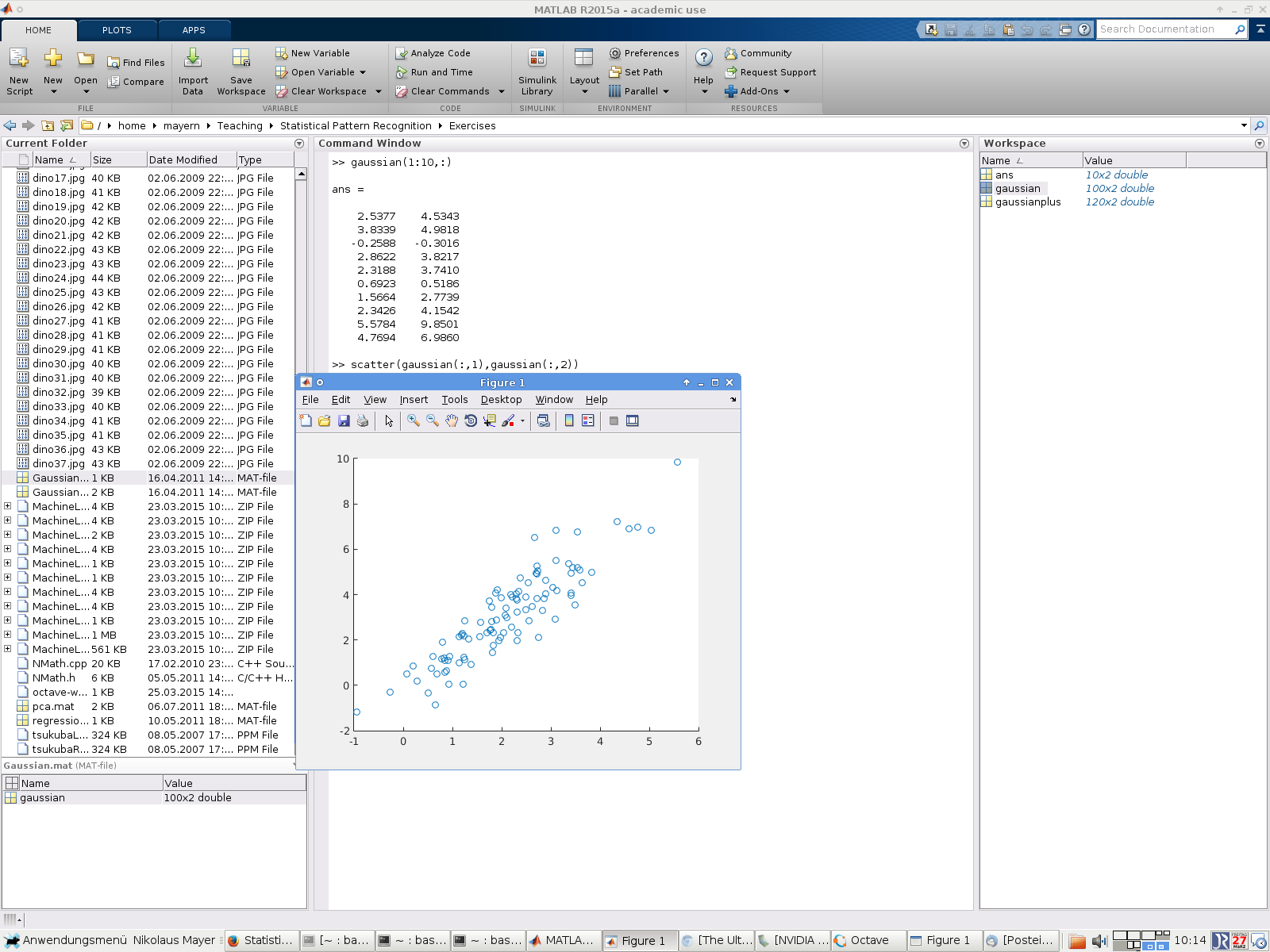
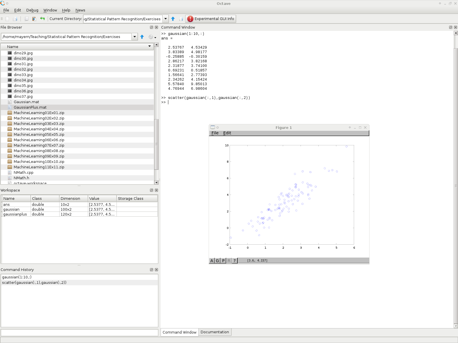
The most comfortable way to get your data into Matlab is to start the program in the directory where you keep the data files. The "Current Folder" file browser built into the Matlab interface lists all files. Double-click on an entry to load the file. Alternatively, type e.g. load('Gaussian.mat'). The "Workspace" view lists all currently valid handles. Inside Matlab's command window, you can navigate just like in a terminal (using ls, cd etc.).
Matlab's worst beginners' pitfall is arguably that it is 1-indexed. The first element 0 of a vector vec = [0 1 2] is accessed by vec(1).
The exercise wants you to "plot the points using plot". While plot(gaussian) works, it won't show you what you actually want to see, which is a 2d plot of the point samples encoded in the given matrix. Instead, call a different version of this function plot(gaussian(:,1), gaussian(:,2), 'o') or do a scatter plot: scatter(gaussian(:,1), gaussian(:,2)).
You can look up commands using the builtin documentation (e.g. edit plot for the plot command) or the online function index. For Octave, use the online function index.
Welcome — this is a landing page for the Statistical Pattern Recognition lecture in the Summer Term of 2015.
If you have any questions, if anything isn't (but should be) working, or if you want to present your results — just ask us tutors, after all that's why we are here. Come see us at our offices or shoot us an email.
The university has a state license for the Matlab computing software that we use for the hands-on exercises. If you want to use your own computer, you can obtain a student license (free of charge; see section 'Software acquisition (Student Option)') from the software shop of the university.
If the matlab command is invalid on a pool machine, try /usr/local/ufrb/MATLAB/bin/matlab.
Instead of Matlab you can also use the free alternative Octave. It is designed with Matlab compatibility in mind, and as far as our exercises go, it can be seen as exactly the same, i.e. it supports the same syntax, functions, structure...
On Linux, install Octave via your package manager or load the latest source package (3.8.2), then install using ./configure && make install (patience — the source is reasonably small but blows up to about 3.5GB during compilation). Depending on your system, you may need to install up to a dozen other dependencies first.
Octave also has a graphical interface very similar to Matlab's, but it is still under development and not yet active by default: Use the command line option --force-gui. Here's how close the two interfaces are: Matlab vs Octave.
The R Project is another open-source software option. While also very powerful, it has a vastly different design and is not as Matlab-like as Octave. Unless mentioned otherwise, all notes on this page apply to both Matlab and Octave, but not to R.